Rationale and background:

Tools for estimating population structure and from genetic data are now used in a wide variety of applications in population genetics. In addition, identifying the degree of admixture in individuals and inferring the population of origin of specific loci in these individuals is relevant for a variety of problems in population genetics. With decreasing costs in sequencing and genotyping technologies, there is an increasing need for fast and accurate tools to infer population structure from very large genetic data sets. However, inferring population structure and identifying the degree of admixture in large modern data sets imposes severe computational challenges. fastStructure is a fast algorithm for inferring population structure from large SNP genotype data. It is based on a variational Bayesian framework for posterior inference and is written in Python2.x (Anil Raj et al., Genetics Jan 2014). It is an efficient algorithm for approximate inference of the model underlying the STRUCTURE program.Variational methods pose the problem of computing relevant posterior distributions as an optimization problem, allowing the use of recent advances in optimization theory to develop fast inference tools. In addition, useful heuristic scores can be used to identify the number of populations represented in a dataset and a new hierarchical prior to detect weak population structure in the data. The variational algorithms are almost two orders of magnitude faster than STRUCTURE and achieve accuracies comparable to those of ADMIXTURE. Furthermore, the results show that the heuristic scores for choosing model complexity provide a reasonable range of values for the number of populations represented in the data, with minimal bias towards detecting structure when it is very weak.

This tutorial will take users through steps of:

1. Launching the fastStructure Atmosphere image
2. Running fastStructure on an test data 

Please work through the tutorial and add your comments on the bottom of this page. Or send comments per email to support@cyverse.org. Thank you.

Part 1: Connect to an instance of an Atmosphere Image (Virtual Machine)

Step 1. Go to https://atmo.cyverse.org and log in with your CyVerse credentials.

Step 2. Create a new project (faststructure) and add some description after log-in.

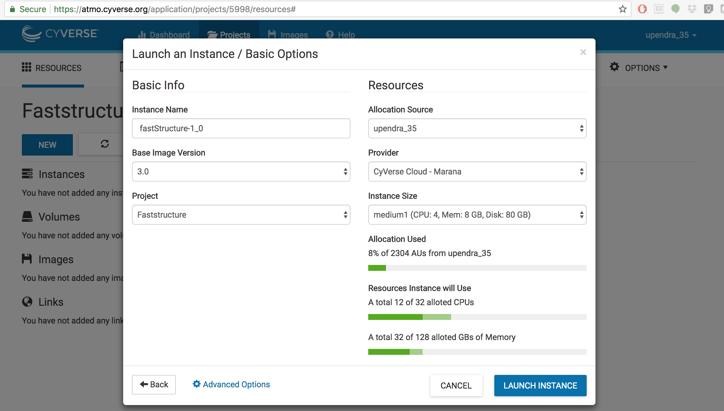
Step 3. Click on the Launch New Instance button and search for fastStructure-1.0 image.

Step 4. Click Launch Instance. It will take 2-5 minutes for the cloud instance to be launched. 

Note: Instances can be configured for different amounts of CPU, memory, and storage depending on user needs.  This tutorial can be accomplished with the medium1 instance size, medium1 (4 CPUs, 8 GB memory, 80 GB root)  

Part 2: Set up a fastStructure run using the Terminal window

Step 1.

• Open the Terminal on mac.  Add the ssh details along with your IP address to connect the instance through the terminal

$ ssh <username>@Ipaddress

• or using webshell

Step 2. Get oriented. 

1. You will find fastStructure software in "/opt" folder. All the dependencies for running fastStructure are located in "/opt/fastStructure" but you need to change the permissions before using it 

$ ls /opt/fastStructure-1.0/
build       distruct.py      fastStructure.pyx  LICENSE      parse_bed.pyx  parse_str.c    parse_str.so  setup.py      test
chooseK.py  fastStructure.c  fastStructure.so   parse_bed.c  parse_bed.so   parse_str.pyx  README.md     structure.py  vars

Step 3. The staged example data can be found in folder "fastStructure/test" within "opt" folder.  List its contents with the ls command:

$ ls /opt/fastStructure-1.0/test
testdata.bed  testoutput_logistic.3.log    testoutput_logistic.3.varP  testoutput_simple.3.meanP  testoutput_simple.3.varQ
testdata.bim  testoutput_logistic.3.meanP  testoutput_logistic.3.varQ  testoutput_simple.3.meanQ
testdata.fam  testoutput_logistic.3.meanQ  testoutput_simple.3.log     testoutput_simple.3.varP

The testdata.bed file (with corresponding test.fam and test.bim) contains genotypes sampled for 200 individuals at 500 SNP loci. There are also other testdata outpuut files. Let's copy the files

$ cd ~
$ cp -R /opt/fastStructure-1.0/test .
$ rm test/*output*
$ ls test
testdata.bed  testdata.bim  testdata.fam

Step 4. Set up a fastStructure test run.  Executing the code with the provided test data should generate a log file identical to the ones in test/, as a first check that the source code has been downloaded and compiled correctly. The algorithm scales linearly with number of samples, number of loci and value of K; the expected runtime for a new dataset can be computed from the runtime in the above log file.

$ python /opt/fastStructure-1.0/structure.py -K 2 --input=test/testdata --output=test/testoutput_simple --full --seed=100
$ python /opt/fastStructure-1.0/structure.py -K 3 --input=test/testdata --output=test/testoutput_simple --full --seed=100
$ python /opt/fastStructure-1.0/structure.py -K 4 --input=test/testdata --output=test/testoutput_simple --full --seed=100

$ ls test
testdata.bed             testoutput_simple.2.meanP  testoutput_simple.3.log    testoutput_simple.3.varQ   testoutput_simple.4.varP
testdata.bim             testoutput_simple.2.meanQ  testoutput_simple.3.meanP  testoutput_simple.4.log    testoutput_simple.4.varQ
testdata.fam             testoutput_simple.2.varP   testoutput_simple.3.meanQ  testoutput_simple.4.meanP
testoutput_simple.2.log  testoutput_simple.2.varQ   testoutput_simple.3.varP   testoutput_simple.4.meanQ

Step 5. Choosing the model complexity: In order to choose the appropriate number of model components that explain structure in the dataset, it is recommended to run the algorithm for multiple choices of K. FastStructure provides a utility tool to parse through the output of these runs and provide a reasonable range of values for the model complexity appropriate for this dataset.

Assuming the algorithm was run on the test dataset for choices of K ranging from 1 to 5, and the output flag was --output=test/testoutput_simple, you can obtain the model complexity by doing the following:

$ python /opt/fastStructure-1.0/chooseK.py --input=test/testoutput_simple
Model complexity that maximizes marginal likelihood = 2
Model components used to explain structure in data = 2

Here the best model to explain the data is 2.

Step 6.  Visualizing the admixture proportions. In order to visualize the expected admixture proportions inferred by fastStructure, fastStructure provided a simple tool to generate Distruct plots using the mean of the variational posterior distribution over admixture proportions. The samples in the plot will be grouped according to population labels inferred by fastStructure. However, if the user would like to group the samples according to some other categorical label (e.g., geographic location), these labels can be provided as a separate file using the flag --popfile. The order of labels in this file (one label per row) should match the order of samples in the input data files.

$ python /opt/fastStructure-1.0/distruct.py -K 2 --input=test/testoutput_simple --output=test/testoutput_simple_distruct_K2.pdf
$ python /opt/fastStructure-1.0/distruct.py -K 3 --input=test/testoutput_simple --output=test/testoutput_simple_distruct_K3.pdf
$ python /opt/fastStructure-1.0/distruct.py -K 4 --input=test/testoutput_simple --output=test/testoutput_simple_distruct_K4.pdf

$ ls
testdata.bed               testoutput_simple.2.varP   testoutput_simple.3.varQ   testoutput_simple_distruct_K2.pdf
testdata.bim               testoutput_simple.2.varQ   testoutput_simple.4.log    testoutput_simple_distruct_K3.pdf
testdata.fam               testoutput_simple.3.log    testoutput_simple.4.meanP  testoutput_simple_distruct_K4.pdf
testoutput_simple.2.log    testoutput_simple.3.meanP  testoutput_simple.4.meanQ
testoutput_simple.2.meanP  testoutput_simple.3.meanQ  testoutput_simple.4.varP
testoutput_simple.2.meanQ  testoutput_simple.3.varP   testoutput_simple.4.varQ

Step 7. Downloading the files using cyberduck.

For a new dataset, it is recommend executing fastSTRUCTURE, for multiple values of K to obtain a reasonable range of values for the appropriate model complexity required to explain structure in the data, as well as ancestry estimates at those model complexities. For improved ancestry estimates and to identify subtle structure, it is recommend executing fastSTRUCTURE with the logistic prior at values of K similar to those identified when using the simple prior.